
This is the third tutorial in a three-part series, providing a use case where a credit card company might benefit from machine learning techniques to predict fraudulent transactions.
If you missed them, catch up with part one and part two.
Now that the data is ready, you’ll train several models to resolve the initial statement. It’s not our intent here to explain those models in detail.
For this final part of the tutorial, you’ll need scikit-learn* (sklearn.) It’s the one of the most useful and robust libraries for machine learning in Python*. It provides a selection of efficient tools for machine learning and statistical modeling including classification, regression, clustering, and dimensionality reduction through a consistent interface in Python. This library, largely written in Python, is built on NumPy*, SciPy* and Matplotlib*.
The Intel® Extension for scikit-learn offers you a way to accelerate existing scikit-learn code. The acceleration is achieved through patching: replacing the stock scikit-learn algorithms with their optimized versions provided by the extension (see the guide). That means you don’t need to learn a new library but still get the benefits of using sklearn, optimized.
The example below will show the benefits.
Training
Which algorithm should you use? The one that best predicts your future data. That sounds simple but selecting the most advanced algorithm doesn’t mean that it will be useful on our data. It’ll be the one that gives you the best results (in test) over the metric we choose. Don’t expect a 100% accuracy because that's not a good sign: Decide in advance what would be an acceptable value (70%, 80%, 90%). Remember to consider how long it takes the algorithm to process the results.
Algorithms
Now you’ll explore two families of algorithms: logistic regression and decision trees. Before diving in, you’ll need a basic understanding of how metrics work and how they can help us to understand the behavior of the model.
Accuracy / Precision / Recall / F1 score
Each metric has advantages and disadvantages, and each of them will give you specific information on the strengths and weaknesses of your model.
Even if the words “accuracy” and "precision” have similar meanings, for artificial intelligence they are two different concepts. When you need to know the overall performance of the model, pay attention to accuracy only. This is defined as simply the fraction of correct classifications (correct classifications/all classifications). It won’t help in cases like this one, where it’s important to get a model that can detect fraud cases because it’s a metric that works to detect all correct predictions regardless of whether they are fraud or not fraud. In other words, accuracy can answer this question: Of all the classified examples (fraud and no fraud) what percentage did the model get right?
Moreover, in AI the term precision considers both true positives (TP) and false positives (FP) (TP/(TP+FP)). This will give you a ratio between hits and errors for each class for positive predictions. In other words, a precise answer to this question: Of the examples the model flags as fraud, what percentage were actually fraud?
Finally, the term “recall” differs to precision because it considers false negatives (FN) (TP/(TP+FN). It gives you more information because it also considers those examples that the model classified incorrectly as no fraud when they are fraud.
In other words, recall answers this question: Of the examples that were actually fraud, what percentage was predicted as fraud by the model?
There’s one more metric to keep in mind called the F1-Score, an average between precision and recall. You’ll get a harmonic mean, which can be useful because it represents both precision and recall represented in just one metric.

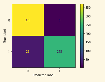
Confusion Matrix
This a table with the combinations of predicted and real values. It shows how many examples are TP, NP, FN, TN.
Now you’re ready to build your models. Depending on which algorithm and framework you're using, there are different ways to train the model. Intel optimizations can help speed them up, too. There are several approaches to consider including regression, decision trees, neural networks and support vector machines among others.
Model 1: Logistic Regression
Regression is a statistical method by which one variable is explained or understood on the basis of one or more variables. The variable being explained is called the dependent, or response, variable; the other variables used to explain or predict the response are called independent variables (Hilbe, 2017)
Regression is a type of supervised learning. Making the model fit can result in slow training but the prediction is fast. It can’t help in scenarios where the relationship between them is not easy to predict (complex relationships).
To understand logistic regression, you need to understand a linear regression first.
Let’s say you would like to predict the number of lines coded based on time coding (1 dependant variable) Image 2. A linear regression will find a function (blue dotted line) that can return a value (lines) when you give your input variable (hours coding), there is a multivariable regression when you have multiple dependant variables, but the concept is still the same. Linear Regression (dotted line) then will return a continuous value (number). It won’t be helpful in this Fraud detection case where you are looking to a classification of “fraud” or “not fraud”.

Image 2
Then, you’ll use Logistic Regression (image 3). It will give you “true” and “false” values (fraud or not fraud). Instead of fitting a line, logistic regression fits an “S” shape which corresponds to a probability value of being “true,” in other words a value between 0 and 1 where the model will consider “true” if it’s higher than 0.5.
To classify, start from an input value marked in green (X-axis), and a line is drawn up to the intersection with the blue line (log reg), with the value in Y-axis as the result for that value. Because the match here is less than 0.5 (0.41) it will be labeled as "fraud." You can calculate all the test values using the same procedure. This is done automatically when you ask the model to "label" your cases.

Image 3
Train
You’ll start training the model, using sklearn API “fit”. It will train the model with X (train data without labels) and y (labels of train data). Pretty straightforward.
clf = LogisticRegression(random_state=0).fit(X, y)
Performance in TRAIN
Once the model is trained, you can take a better look at its performance and start predicting the labels for the “train” dataset. Note: sklearn will provide you with the label (1 or 0), you can use predict.proba to see the probabilities.
y_pred= clf.predict(X)     # It will give the

target_names = ["FRAUD","NO FRAUD"]


print(classification_report(y, y_pred,target_names=target_names))

As you can see, it’s at 95% percent accuracy. It means that the model can correctly identify most of the examples. Since our goal is to have a model capable of generalizing on unseen data, you can imagine that high levels of accuracy in training is related to good results, right?
However, that's not the case. High levels of accuracy in training means that the model has a perfect understanding of the data provided (train). Test cases are not necessarily equal to train examples -- the accuracy there could drop from 95% in training to ~50% in test.
For example, if you’re building a model to detect cows and you get the 100% accuracy in train, when you move to test it won’t be able to detect a slightly different cow, your model is not able to generalize. Known as "overfitting,” there are multiple ways to avoid it. Random samples, equally distributed datasets, cross-validation, early stopping or regularization between other techniques are useful.
Note: It’s a good thing when you get high levels of accuracy in "test" (inference)!
## Confusion matrix

from sklearn.metrics import plot_confusion_matrix


#y_pred = clf.predict(X)

plot_confusion_matrix(clf,X, y)
Performance in test:
This next step is known as inference. Now that you’ve trained the algorithm trained, you need to verify the performance on unseen data. You’ll test with the same metrics you did for training, but it's time to start thinking about how this model will perform in your solution. For example: Will the implementation consist of thousands of inferences at the same time? In that case, you’ll have pay attention to the time the algorithm takes to give you the result (fraud vs no fraud), you will probably choose the algorithm that gives you the result faster, normally combined with analysis of the hardware and software optimizations available.
test_pred=clf.predict(test)


target_names = ["FRAUD","NO FRAUD"]


print(classification_report(y_test, test_pred,target_names=target_names))

plot_confusion_matrix(clf,test, y_test)

As you can see there’s a drop in metrics results when making the inference. It’s still a good predictor but it makes mistakes, and you should evaluate how important are those mistakes are overall. As a guideline, a model with 85% precision on fraud cases is not bad at all.
Model 2: Decision Trees
A decision tree is a type of supervised learning. A decision tree can help you decide a question like: “Is this a good day to code?” The inputs could be factors such as time of day, external noise, and hours coding. The algorithm will find in the training data the best split to classify if it’s a good day to code or it doesn’t. The result might look like the following:

Image 4
The concept was first introduced by Leo Breiman in 1984 (Breiman, 2017). Here you'll use Random Forests* which is a decision tree-based algorithm that builds several trees while training and selects the best to use. XGboost*or LightGBM*, and many others share the same concept behind with different approaches and techniques to build the decision trees.
Decision trees can give a very intuitive explanation about how the decisions were made. Keep in mind, though, that it might be inadequate when you’re looking to predict continuous values.
Train
There are multiple parameters you can use to train your Random Forest algorithm. Here we’re using a “classifier” to fine tune it. In this case, you’ll keep it as simple as possible to get decent results. Start with a different max_depth value. You’re defining the depth of the decisions tree (longer can be better but could overfit the model.) Here you’ll use six, but you can try with different values to see how performance changes.
clf = RandomForestClassifier(max_depth=6, random_state=0)

clf.fit(X, y)
Performance in TRAIN
Check the performance in train. The results seem slightly better than logistic regression.
y_pred_RF= clf.predict(X)

target_names = ["FRADUD","NO FRAUD"]


print(classification_report(y, y_pred_RF,target_names=target_names))

Performance in test (inference):
test_pred_RF=clf.predict(test)

target_names = ["FRAUD","NO FRAUD"]

print(classification_report(y_test, test_pred_RF,target_names=target_names))

After training two simple models you can expect decent performance (in test) on both.
Conclusion
In this tutorial, you’ve trained a model to detect possible fraudulent transactions with a few different models. The tutorial covered the main concepts around how to train a model that can be used to detect fraud, you’ve prepared/transformed the data and you’ve selected some algorithms to train it.
With these results, you can now decide which model to use based on metrics, keeping in mind that execution time is an important topic when implementing the algorithm. Your model is almost ready to implement in your application. The next step is to optimize container packing (more on that here), then integrate it into your solution to take advantage of the insights the model will give you.
The model you trained in this tutorial can potentially save your company time and money by proactively spotting transaction fraud. A recent Gartner report notes the uptick of banks using AI in growth areas such as fraud detection, trading prediction and risk factor modeling.
To see the Intel toolkits in action and how they can speed up the process, check out the entire notebook on GitHub.
References
Breiman, L. (2017). Classification and regression trees. Routledge.
Hilbe, J. M. (2017). Logistic Regression Models. Taylor & Francis Ltd.